77-420 Online Practice Questions and Answers
Modify the text in the title.
Cell A1.
Text "Math 1080 - Section 3 Assignments"
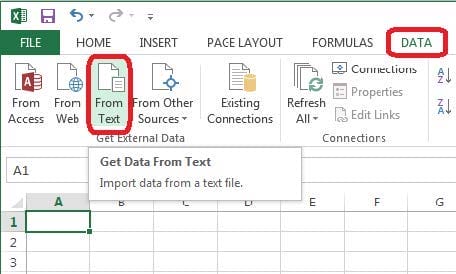
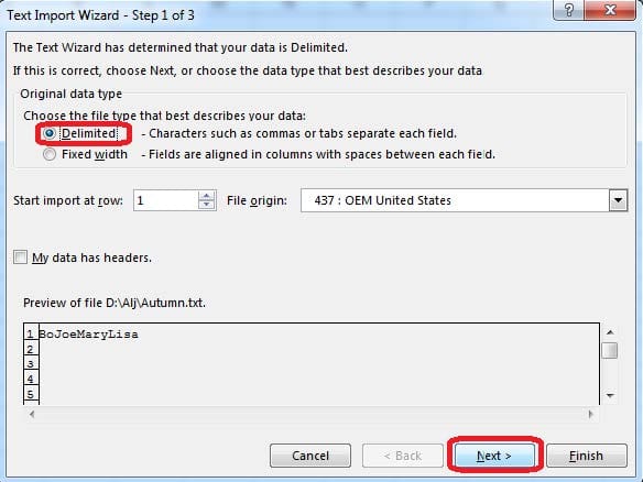
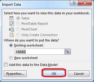
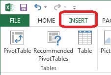
Insert data from a text file.
Cell A1.
File source Autumn.txt
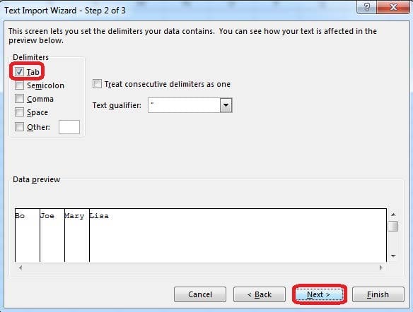
Tab-delimited
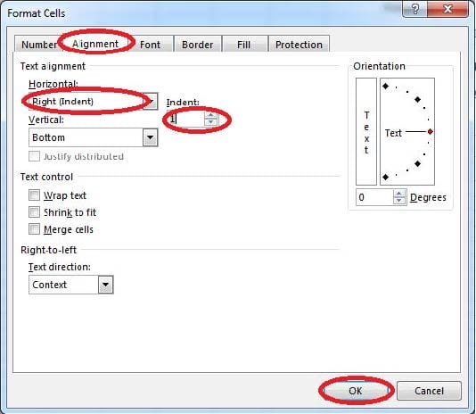
Modify the cell alignment settings.
Cell range B3:B25
Horizontal: Right (Indent)
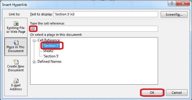
Create a hyperlink to another worksheet.
Cell A2.
Cell reference "A3"
Sheet reference "Section 3" worksheet.

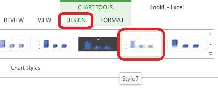
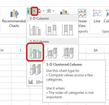
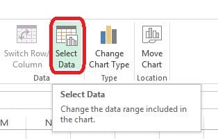
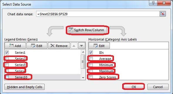
Create a chart. To the right of the data Chart 3-D Clustered Column Exclude all filtered rows Horizontal Axis Labels: "IDs" column in table Series 1: "Zero Scores" column in table.
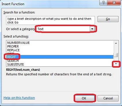
Insert the instructor's name for column B.
Cell B5.
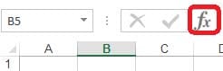
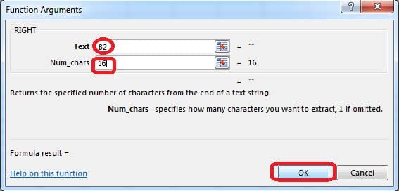
Use Function RIGHT
Text: B2
Absolute reference
Num_chars: "16"
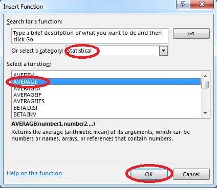
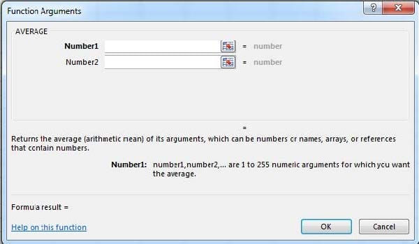
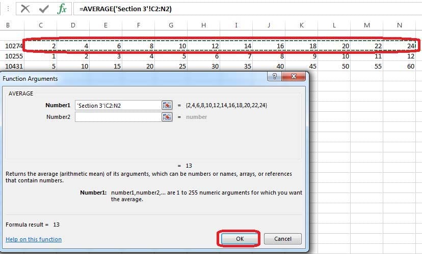
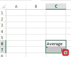
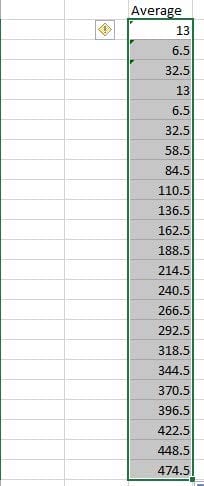
Formula. Find the average of each student's homework scores.
Cell range C7:C29
Use Function AVERAGE
Number 1: all homework for each student on "Section 3" worksheet "22-Aug 12-Dec"
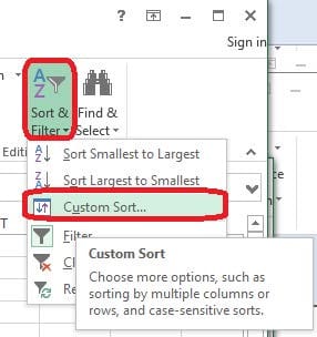
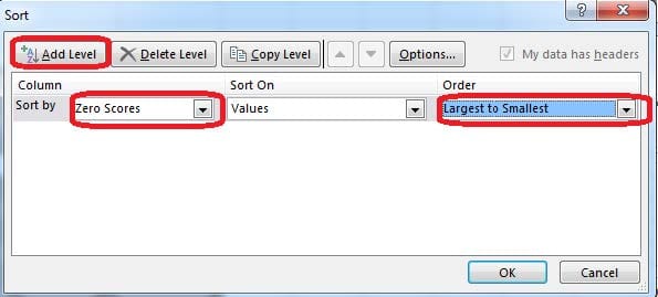
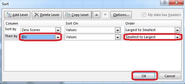
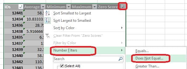
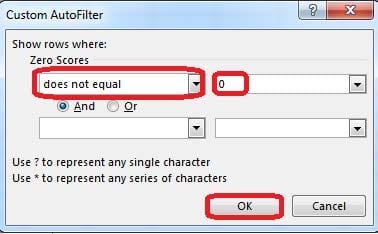
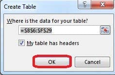
Sort and Filter. Apply a sort and a filter to the table. Cell range B6:F29 Sort Column Zero Scores Order Largest to Smallest Column IDs Order Smallest to Largest Filter Hide students ids with no zero scores.
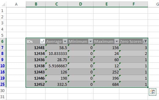
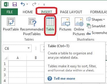
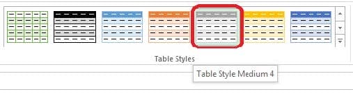
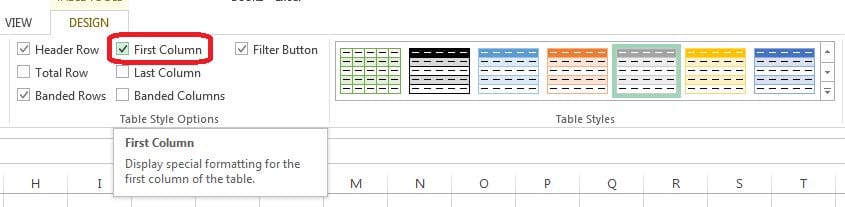
Create a table and modify the table styles. Cell range B6:F29 Table Style Medium 4 Enable the First Column Style
Why select/choose certbus.com?
Millions of interested professionals can touch the destination of success in exams by certbus.com. products which would be available, affordable, updated and of really best quality to overcome the difficulties of any course outlines. Questions and Answers material is updated in highly outclass manner on regular basis and material is released periodically and is available in testing centers with whom we are maintaining our relationship to get latest material.
![]()
![]()
Copyright © 2004-2025 certbus.com, All Rights Reserved.